ECC Technical
Information about the theory of Earth Current Communications.
Basic Theoretical Principles
The fundamental principle of ECC utilises the inherent "resistance" of the earth. Signals are detected by a distant receiver by currents induced to flow through the earth at the receiver by the transmitter causing a potential difference to exist between points in the earth at the receiver. This is possible because current forced to flow between two earth rods at the transmitter does not all flow in a straight line between the two rods. Some proportion of the current flows in arcs away from a straight line between the two rods. The more pronounced arcs trace out a path well away from the direct line between the two rods. It is the current in these pronounced arcs that can be used to communicate information to locations well outside the direct line between the two rods.
NOTE: To (hopefully) avoid confusion the term "probe spacing" refers to the spacing between the two individual rods of a probe pair, while "distance" or "range" refers to the distance between probe pairs (i.e., the communication path).
One principle that is useful to appreciate is that the "resistance" between two earth rods or probes is an apparent resistance. That is, it can be calculated from the voltage and current applied to the probes as would normally be done for an actual resistance component (resistor). However, further analogy is not wise. For example, if one were to apply a voltage of 100V between two probes spaced 100 metres apart and measured a current of 1A the apparent resistance is 100 ohms (R = V/I = 100/1 = 100 ohms). It might seem reasonable to expect that if the probes were now placed 200 metres apart the doubled distance would mean a halving of the current to 0.5A for an applied 100V giving a resistance between the probes of 200 ohms. In fact the current would still be close to 1A (assuming the ground conditions are the same under the 200m layout as the 100m layout). That is, the apparent resistance is still close to 100 ohms. So the behaviour is not the same as tacking resistors in series. This may be explained by considering that the more the current paths arc away from the direct line between the two probes, the more parallel paths there are for the current to flow. Using a gross simplification - when the distance is increased between the transmitting earth probes, the increase in direct line resistance is cancelled out by reduction in resistance due to an increasing number of effectively parallel paths made available.
Be aware that the above description and that which follows are general. Individual installations will differ greatly due to local soil type and moisture conditions. In other words, it may be found that the resistance remains reasonably constant with increased earth probe spacing, but don't be surprised if does not.
The relationship between resistance R (V/I) and resistivity of a material (Rho) is:-
R = Rho * L / A
where L is the length of the material and A is the cross-sectional area. In the case of increasing spacing of earth probes, as L is increased, the effective cross-sectional area A available to carry current increases as well. Therefore the ratio L/A tends to remain constant leaving the actual value of resistance largely dependent on Rho, the resistivity of the soil. Note that if the soil under the probes is not homogeneous then the apparent resistivity measured in a survey will change with changing probe spacing. This is because as the probe spacing is increased the current flows deeper and therefore is affected by the characteristics of the soil at depth. For example, if the soil beneath the probes is layered with a high resistivity layer near the surface and a lower resistivity layer deeper down, then the apparent resistivity will fall as probe spacing is increased. Conversely, for a low resistivity layer near the surface and a high resistivity layer deeper down, the apparent resistivity will rise with increased probe spacing. Finally, for three layers starting with a high Rho layer near the surface, then a low Rho layer in the middle, then a high Rho layer as the deepest, the apparent resistivity will firstly fall with increasing probe space as the middle layer increases in influence and then rise again as the bottom layer increases in influence... So R can basically wander about as probe spacing is increased depending on the non-homogeneity of the soil beneath the probes.
Another way of looking at this effect is imagine the area that the current has to pass through right adjacent to the earth probe. This area is essentially the cylindrical surface area of the rod which for a rod of 10mm diameter and 1.2m length is 1.2 * (PI * 0.01) square metres = 0.038 sq m. At a distance of 0.5m from the rod the area is a cylinder (1.2 + 0.5) * (PI * (0.01 + 0.5)) = 2.72 sq m. At a distance of two metres from the rod the area available for current flow is (1.2 + 2) * (PI * (0.01 + 2)) = 20.2 sq m. So the resistance presented to the current right next to the rod compared to the resistance present at a distance of 2m is in the ratio of (20.2 / 0.038) = 532:1 assuming the resistivity remains the same. Basically the resistance to general earth is almost totally governed by the soil resistivity within about 3m to 5m of the earth probe and the rod-to-earth contact area. when trying to effectively double the rod-to-earth contact area by adding an extra rod and electrically shorting the two rods together (making 4 rods altogether), the distance between two paralleled rods should therefore be at least 6m to 10m. If the rod spacing was originally a few 10s of metres then this obviously becomes difficult. A better method of of doubling the rod-to-earth contact area is to double the length of the earth rod. Note that in terms of volume of steel (closely related to cost) it is better to double the length than to double the diameter of the rod. Both give a doubling of surface area but doubling the diameter multiples the volume of the rod by 4, while doubling the length only multiplies the volume of the rod by 2. Also it is probably easier to hammer in a rod twice as long than it is to hammer in a rod of twice the diameter. Plus the longer rod will reach down to more moist soil not affected by ambient weather conditions.
By the way, if a 100m capped length of PVC pipe were to be filled with local soil and the apparent resistance measured between the ends and then the measurement repeated with a 200m length filled with the same type of soil, then it would be found that the 200m exhibits roughly twice the apparent resistance of the 100m length. Here the length of the path L increases while the cross-sectional area A is held constant by the constraint of the insulating pipe.
The actual apparent resistance measured at any transmitting site is largely governed by the efficacy of the earth probes (how well they couple into the earth) and the resistivity Rho of the earth between the probes down to a depth roughly equal to one-third the distance between the probes.
The dependence of the apparent measured resistance (as calculated by the voltage applied to a pair of earth probes divided by the current flowing between these earth probes) mainly on the "contact" resistance of the probes to earth is the reason that geological surveys use a separate current injection probe pair and a separate voltage capture probe pair. By using the current reading only from the transmitter probe pair and measuring voltage from a separate probe pair the effect of the voltage drops across the "contact" resistance of the probes is eliminated. This is because the measurement of current injected is not affected by the voltage drop across the injecting probe pair and by use of high impedance (very low input current) measuring devices across the voltage receiver probes the voltage drop across the receiver probe contact resistance is virtually eliminated.
For a one-way ECC link it would seem important to have good transmitting earth probes with low contact resistance to minimise the power required to achieve a given current magnitude, while the receiving earth probes can be of lesser quality provided the receiver presents a high impedance load to the receiving earth probe pair.
The received voltage as measured between the distant receiver electrodes is directly proportional to the product of the induced earth current at that point and the resistivity of the earth between the receiver probes at that point down to a depth roughly equal to one-third the distance between the receiver probes. The induced current flowing in the ground at the receiver probes is directly proportional to transmitter current and inversely proportional to the cube of the distance between transmitter and receiver (ouch !!!).
A great deal of information can be inferred about ECC from the information associated with geological and archaeological surveys that employ DC resistivity surveys to locate subterranean objects or features. These employ a number of probes in various configurations. Each of these configurations have strengths and weaknesses for resistivity surveys, but the only configurations of interest to ECCers are the dipole-dipole (in-line) and the equatorial dipole-dipole (broadside or goal posts) configurations. These two resistivity survey configurations are the only ones where the receiving probe pair lies outside the transmitting probe pair. The "geometric factor" of each of these two configurations gives a measure (as applied to ECC) of the received signal strength at a distance. The following diagram is from the documentation of the freeware program RES2DMOD ver 2.2 provided by M.H.Loke.
Here C1,2 are the transmitter probes and P1,2 are the receiver probes. Interestingly, the Equatorial Dipole-Dipole configuration seems to be the assumed configuration of choice (except for several experimenters). However, if the "Geometric Factor" relationship is correct, the Dipole-Dipole (inline) configuration has an advantage of about 12dB over the Equatorial Dipole-Dipole configuration. Mark (G0KZZ) reports that he has observed this advantage experimentally over short distances. Of course, the inverse distance-cubed factor means that an extra 18dB is required to double the distance, so the 12db advantage mentioned only gets an increase in distance by a factor of 1.6 times.
The relationship for the voltage V received between P1 and P2 using the above configurations is:
V = Rho * I / k
where I is the current driven between C1 and C2, k is the geometric factor and Rho is the resistivity of the earth between and below each of the probe pairs (location identified by 'a' in the diagram above). The resistivity of the earth between the probe pairs (location identified by 'na' in the diagram above) has a lesser effect.
ECCers are not really interested in quantifying the resistivity of the earth, but rather the interest lies in maximising the received voltage V relative to background noise for any given input power and distance 'na'.
One thing that may be significant from the field of resistivity surveys - fundamentally the excitation current used there is DC, but because of self-polarisation potentials at the probes and the effect of Telluric currents, it is common for these surveys to use AC excitation. Of particular note is the mention that such AC is usually low frequency (< 20Hz) to replicate the results of DC surveys. This may indicate that there may exist some significant benefit in using frequencies below 20Hz for ECC.
Theoretical Attenuation versus Distance
The diagram below shows the theoretical relative attenuation of a signal versus distance for both the Equatorial Dipole-Dipole (broadside) and the Dipole-Dipole (inline) configurations. The attenuation has been referenced to the late John Taylor's 10Km record (assuming the Equatorial Dipole-Dipole configuration was used for his 6kHz ECC tests) as the 0dB point with probe spacing of 100m at both the transmitter and receiver end. It shows 18dB attenuation with each doubling of distance. That is, if data can be received at 10Km with a certain S/N ratio, then it would require an 18dB improvement in path gain to get the same S/N ratio at 20Km (assuming the same background ground noise at both locations). This can be an increase in power by 18dB (increase power by 63 times) or a reduction in bandwidth by a factor of 63 times.
Note the diagram below is a plot of signal level, not S/N.
The diagram below shows how increasing the spacing between probes at both the transmitter and receiver increases the distance for the same signal level or strength. The heavy circle marks the 100m probe spacing/10Km distance point.
The relationship for distance gain factor versus probe spacing for the same signal strength/level is:-
Df = (spacing factor)2/3
For example, doubling the spacing between the earth probes (spacing factor x2), gives an increase in distance factor of:-
Df = (2)2/3 = 1.59
Trebling the spacing gives:-
Df = (3)2/3 = 2.08
From this it can be seen that theoretically trebling the spacing between the earth probes gives roughly the same increase in distance as a 19.1dB increase in transmitter power (going from, say, 10W to 813W) or dropping from 100Hz bandwidth to 1.2Hz bandwidth.
These theoretical calculations show an advantage of 11dB to 12dB of the inline configuration over the equatorial configuration for distance/spacing ratios of greater than 50 or so. This advantage is equivalent to a doubling of the spacing at both ends or a quadrupling of spacing at the transmitter end alone. At any given distance, a lift in 12dB in S/N could be the difference between successful reception or no reception. Or, for the same S/N, an increase in distance covered by a factor of 1.6 times.
Practical ECC Communications
The theoretical treatment discussed elsewhere is derived from formulae applicable to resistivity survey applications. As mentioned elsewhere, ECCers are more interested in the communication link budget side of the equation. The attenuation and distance graphs do not include background ground noise in the real environment. When operating in the real world environment ECC communications are subject to interference and background noise limitations as in other modes. The factor which determines whether data can be received at distance is not the signal strength alone, but the signal-to-noise ratio. In the theoretical calculations the probe spacing variations are assumed to occur at both the transmitter and receiver. In practice, it could be imagined that once the signal from the receiver probes (wanted signal + background noise) is high enough to swamp the receiver noise, further increases in spacing at the receiver will not improve the signal-to-noise ratio. Further increases in probe spacing at the receiver above the level necessary to swamp the receiver noise are expected to be a wasted effort as it will raise both the in-ground background noise and the signal by the same amount. Therefore, the S/N will remain the same as illustrated by the following...
S/N = Ps / (Pr + Pb)
where Ps, Pr and Pb are signal, receiver and ground noise respectively. At low receiver probe spacings where Ps and Pb << Pr then increasing the receiver probe spacing improves the S/N. At some spacing the level of Ps and Pb >> Pr and the signal-to-noise ratio reduces to:-
S/N = Ps / (Pb)
At this point the S/N does not improve with increased receiver probe spacing. The actual probe spacing at which S/N is not improved by increased receiver probe spacing depends on the level of the background ground noise at the receiver and the noise floor of the receiver - the higher the background noise and the lower the receiver noise - the smaller is the required spacing at which further increases in spacing do not improve S/N. However, increasing the spacing at the transmitter end should increase the signal-to-noise ratio. It is suspected the increase in signal level will be not directly proportional to the square of the transmitter spacing increase, but just directly proportional. That is, holding the receiver spacing constant and doubling the transmitter probe spacing should only give an increase in distance factor of:-
Df = (2)1/3 = 1.26
Therefore, for a Df of 2.08 it is suspected an increase in the transmitter probe spacing by a factor of 9 is needed to get the equivalent range distance increase as provided by a 19.1dB increase in power. So starting with a probe spacing of 10m at the transmitter (and assuming the receiver probe spacing is sufficient to give enough signal + noise to override the receiver noise) an increase in the probe spacing at the transmitter to 90m should provide the same range distance increase as a 19.1dB increase in power.
This asymmetry of the importance of size between the transmitting and receiving probe extent is not unlike the requirements for receiving LF signals. For LF, while it is important to make the size of the LF transmitting antenna as large as practicable to get as much signal out as possible, the LF receiving antenna only needs to be large enough to capture enough signal + noise to override the LF receiver noise.
Deep Probes
The formula used by resistivity studies shows a direct dependence on received voltage on the injected transmitter current. We are curious to know if the techniques used in providing low-impedance earthing systems (e.g., lightning protection systems) are relevant for ECC. In particular whether, in fact, injecting current into low impedance deep probes is better for distant reception by shallow receiver earth probes than shallow transmitter probes. By deep we mean deeper than several metres - some earthing system installations talk about driving probes over 30m down to get to impedances to general earth of a few ohms. We are curious whether the increased current for the same power input due to the low impedance of the deep probes translates into better range or whether some other effect comes into play.
Probe Spacing and Directivity
It is believed that the effect of spacing between probes as far as directivity is concerned is similar to a small LF loop antenna where changing the size only effects the captured signal level, but not the shape of the directional response. Receiving ECC signals is a matter of capturing the potential difference between two points caused by the flow of current through the resistance of the earth. For maximum signal the receiving earth probes need to be placed along the line of the direction of the current flow. Theoretically, if they are placed at right angles to the flow then they are connected to points of equal potential and therefore will capture no signal. This principle may be used to null out an interfering signal in the same manner as magnetic loops are used in the LF bands, that is, improving S/N by placing a noise source in a null (at right angles to the line between the probes). In practice (especially for deep probes) it probably will not be possible to place the noise source in a null for the full length of the probe as current direction can be expected to vary with depth. Besides, it is not practical to align probes driven into the ground. Perhaps an optimum fixed receiver installation would be a number of rods formed into a circle to allow selection of the pair of rods which has the best pickup of signal versus rejection of interference. The diameter of the circle should be sufficient for the background noise to override the receiver noise as discussed above.
Another possibility suggested by Mark (G0KZZ) is to use a vertical triangular loop to allow ground currents to induce current in the lower leg as shown below. This would allow an easy way of rotating the orientation of the 'antenna'. Of course the sloping sides will have an opposing current induced, but because they are further away from the ground current they should not be of sufficient magnitude to cancel the lower leg current. It would be expected that because of this effect, the loop would be less sensitive to deeper currents as the difference in spacing is smaller as a proportion to the depth of the current.
The loop might be un-tuned for lower frequencies or tuned for higher frequencies.
Effects of Local Resisitivity
It is unclear whether for a given transmitter probe spacing it is better to have transmitter probes in low resistivity soil (generally corresponds to higher current for a given power input) or in high resistivity soil (generally corresponds to lower current for a given input power). This is because that although low resistivity soil allows more current to flow between the probes for a given input power, this higher current can more easily flow in a direct line between the probes and less fans out. Conversely, for high resistivity soil less current flows for a given input power, but the current is forced to fan out more due to the higher resistance of the direct path. Mere armchair conjecture on our part here... And of course the resistivity of the soil under transmitter probes is more than likely to be different from the resistivity of the soil under the receiver probes in ECC applications where ranges are over 5Km. How this all pans out in terms of communication path attenuation is just waiting to be determined by actual experiments.
Signal Environment
To avoid confusion the term "probe spacing" refers to the spacing between the two individual rods of a probe pair, while "distance" or "range" refers to the distance between probe pairs (i.e., the communication path).
ECC Signals
Communication via ECC relies on the principle of electrical current flowing through the earth causing a voltage drop across the bulk resistivity of the earth mass between the receiving probes. The desired ECC signal is received at a distance by the transmitter inducing earth currents local to the receiver. For the purposes here the frequency range of interest is confined to 0 - 20kHz.
Man-made Earth Currents
As well as the desired ECC earth currents there are many other man-made sources inducing current to flow in the earth. The predominant source in populated areas is the mains electricity source earth current (the mains supply frequency is commonly 50Hz or 60Hz). If the load currents on the main supply were purely sinusoidal then this unwanted interfering signal would be confined to the mains fundamental frequency. Unfortunately many loads presented to the mains supply are commutated and this results in harmonics (mostly odd) of the mains frequency extending, in some cases, up to 5kHz to 8kHz. With the addition of various utility modulation schemes (e.g., off-peak switching tones) there is a whole range of man-made interfering currents to be dealt with in ECC reception. Passing electromagnetic waves induce currents in the earth as well allowing reception of VLF (and above) transmissions.
Natural Earth Currents
Magnetic storms and associated currents in the ionosphere also induce currents in the earth. Whistlers and tweeks as well as lightning pops can be heard in an ECC receiver of sufficient bandwidth.
Received ECC Signals
The following spectrograms and sound files show the nature of the signals received by an ECC system.
Here is a typical sound file of ECC signals (56 kBytes). The predominant 50Hz (+ harmonics) hum can be heard. The spectrogram below in Figure 1. shows the harmonics extend right up to 3400Hz. Note that the even harmonics (100Hz, 200Hz, 300Hz,...) are 20dB below the odd harmonics (50Hz, 150Hz, 250Hz,...). As the mains frequency wanders about with load changes, so the harmonics wander about. At higher frequencies it is not possible to find a place free of a wandering harmonic as the ranges of successive harmonics overlap.
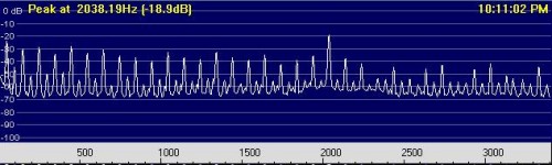
Figure 1. - Spectrogram from 0Hz to 3400Hz
Notice the peak at 2038.19Hz (not that accurate as the bin width is about 5.5Hz) which is the test signal used in one of the scale model tests.
The spectrogram below in Figure 2. shows the range from 0Hz to 106Hz. Here at this narrower bin bandwidth we see the 99.6Hz even (2nd) harmonic is about 30dB below the fundamental 49.8Hz. The broader and stronger peak at 97.5Hz to the left of the 99.6Hz harmonic is of unknown origin.
There is a nice noise valley in the 70Hz to 80Hz range and this is also free from mains harmonics. Also mains modulation products are not present in this range. It is for this reason (and for reasons of the ready availability of cheap high-power low frequency transformers) that a frequency of between 70Hz and 80Hz has been initially chosen as the ECC communication frequency.
As an exercise in serendipity, the ECC Channel frequency of 78Hz has been chosen as a tie to another old technology - the vinyl record 78s.
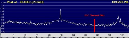
Figure 2. - Spectrogram from 0Hz to 106Hz
Mains Interference Rejection Filtering
To reduce the level of mains generated interference we can use a comb rejection filter. This type of filter produces attenuation notches at the mains frequency and its odd harmonics. A simple off-line method of doing this is to make two copies of the file to be filtered. Move the data from one file back in time by the amount of a half-cycle of the mains fundamental frequency (in the above spectrum which shows a mains frequency of 49.80Hz this amounts to introducing a silence of 10.04 ms into the front of one file). Then add the two files. This has the effect of adding 180 degrees out-of-phase signals for the mains frequency and its odd harmonics only - leaving other frequencies largely unaffected. The result of this filtering on the previous unfiltered sound file (56Kbytes) can be heard in this new filtered sound file (56Kbytes).
The spectrograms of the filtered sound file are below...
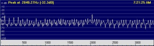
Figure 3. - Spectrogram from 0Hz to 3400Hz - Comb Filtered
The above spectrogram in Figure 3. shows the result of the crude comb filter (not very effective as the audio application only allowed the insertion of 10.1ms - not 10.04ms). The 2040Hz signal has been clobbered to some extent as it is roughly near an odd harmonic of the 49.8Hz mains frequency. Obviously if you wanted to use frequencies up at these frequencies you would pick a frequency mid-way between two mains frequency harmonics. Note how the odd harmonics have been attenuated relative to even harmonics by about 35dB (from 20dB above to 15dB below). Note also this degree of odd harmonic attenuation is only maintained from 0Hz to 400Hz or so. This is because the error in the time delay as noted above becomes a larger error in phase at the higher frequencies.
The spectrogram below in Figure 4. shows the reduction of the fundamental 49.8Hz from 30dB above the 99.6Hz second harmonic as shown in Figure 2. to about 16dB below the 99.6Hz second harmonic as shown in Figure 4. This corresponds to an effective mains fundamental frequency attenuation of about 46dB.
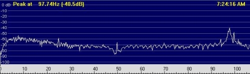
Figure 4. - Spectrogram from 0Hz to 106Hz - Comb Filtered
Practical Implementation of Filtering
In practice the use of a comb filter in real-time makes for a complex implementation. Considering the initial band of frequencies of interest is from 70Hz to 80Hz it would be simpler to implement an analog T-notch filter centered on the mains frequency (50Hz or 60Hz) followed by an analog low-pass filter with cutoff frequency of about 85Hz. A typical spectrogram of this combination is shown below in Figure 5. Because the sound file now contains only frequencies below ~ 85Hz you will need to listen with a good set of headphones or a speaker system with good low frequency response.
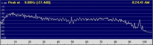
Figure 5. - Spectrogram from 0Hz to 106Hz - Comb Filtered + Lowpass Filtered (fc=85Hz)
If the level of 50Hz or 60Hz mains is low enough (for example - the level shown in these sound files) the dynamic range of a digital recording device (e.g., a MiniDisc recorder or the soundcard input of a PC) of about 96dB will be sufficient to prevent overload on the 50Hz signals while still allowing signals down to the noise floor to be captured. In this case it would only be necessary to provide a lowpass filter (fc= 85Hz) without the T-notch filter. As an illustration of this see the spectrogram below in Figure 6. which shows a 50Hz mains signal (no comb filter) along with a simulated 78Hz ECC signal and the noise level existent at the test site location in the backyard of a semi-rural property.
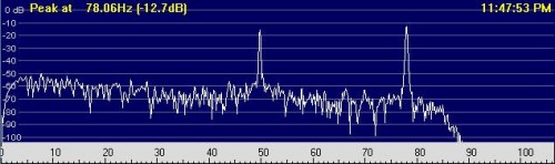
Figure 6. - Spectrogram from 0Hz to 106Hz - Lowpass Filtered (fc=85Hz) + 78Hz ECC Signal
More Detailed Analysis
It would be an advantage to take a longer measurement (say 24hours or more) using a spectrograph and averaging. This would give a good estimate of the probability of encountering interference over the initial frequency range of interest (70Hz to 80Hz). The above spectrograms are generated from sound data of about 14 seconds duration - therefore they are only "snapshots" of signals existent in that epoch. A longer analysis will give a better idea of the statistical likelihood of encountering interference.
Receivers
As the frequency range of interest covered here is 0 - 20kHz, any modern audio recording device is useable to receive ECC signals. At home this could be the soundcard installed inside a PC and in the field it is convenient to use a laptop (for real-time processing) or a MiniDisc for recording signals for later analysis. If the signals received are not of sufficient amplitude a simple audio preamplifier can be used to boost signal amplitude to a level suitable for the recording device. A small transformer can be used to isolate and provide some step up in voltage.
Using a soundcard to receive ECC signals allows all manner of processing via the many audio processing applications available. These include filtering and various other manipulations of the audio data as well as communication link software such as JASON.
Some sort of speaker output (or headphone circuitry with transient limiting to protect the ears) is useful to monitor the received signal especially in the field while conducting experiments.